Chapter 3 Data
3.1 Sources
As mentioned in the previous chapter the data is made available, collected, and maintained by the Internal Revenue Service (IRS).
The primary source of this migration data is derived from Form 1040 which is filed by residents of the United States of America. The tax return data of an individual are matched based on their Tax Identification Number (TIN). After the matching procedure is completed, these are classified into one of 4 categories :
Non-migrant returns,
Migrant return - different state,
Migrant return - same state - different county,
Migrant return - foreign
The data file that we chose for our analysis is the master migration file which contains the migration patterns and data for all the states spread over a span of 5 years from 2016 to 2020 over different age groups.
One of the key issues that we faced while interpreting the data was a large number of categorical variables. Age, Income, and Type of migration were all provided as categorical variables and in a very haphazard manner. These variables were organized in a very unorderly manner and it was very difficult to analyze the data belonging to different categories. Hence, we decided to convert the data frame into the tidy data frame format (more details on this are provided in the next section).
The data file which we used for analysis contains the following variables:
State_code – This column indicates the integer code of the state
State – This column indicates the name of the state.
Returns – This variable indicates the number of households that filed their returns
Individuals – This variable indicates the total number of individuals
AGI_Year1 / AGI_Year2 – These two variables indicate the average gross income (income after deduction of taxes, dividends, etc) on the 2 returns that are filed which are used to identify the migration status. All the AGI amounts are reported in thousands of dollars.
Age – This variable indicates the age category of the individual filing the return
GTI – This variable indicates the gross total income of the individual filing the return
Status – This variable indicates the migration status of the return
Year – This variable indicates the year in which the tax return was filed.
One anomaly we noticed while exploring the data is that the data collection is not consistent in District of Columbia (D.C). There were a few returns filed for certain age groups. On the same note, because D.C. does not have any counties, the values for in-state migration are equivalent to zero.
In addition to the master data file, we also used the state data frame from the maps library. We leveraged this file to obtain the coordinates to plot the various states of the country.
3.2 Cleaning / transformation
For this process, we had to change the structure of the data as it was presented as an .xlsx file with different groups under several layers of merged cells. Using the tidy approach of “one variable per column and one observation per row”, we turned 143 columns into 11, while keeping the core information intact.
Excluding demographic data, our dataset had four core columns of information: number of returns, number of individuals, AGI 1 and AGI 2. These were repeated for each each age group and migration flow status combination. Through the data cleaning and transformation process, we created new columns to flag Age and Migration Status, instead of having separate sections of the file for each. This allowed us to append rows horizontally instead of vertically. Similarly, instead of having a different dataset per year, we collapsed these into one by creating a “Year” column into the main dataframe for the 5 years that we will be evaluating.
The “Total” group was also removed as it was occupying unnecessary space and becoming confusing when extracting summary statistics in R as it would have incorrectly inflated these metrics. We took a similar approach where State was labeled as “Total”.
With these arrangements, the dimensions of our dataframe changed from having 5 datasets 416 x 143 to one dataset 54,600 x 11.
Transformation
Our data contains different demographic information that were initially imported as “character” class type. In order to correctly process and visualize the different groups, we transformed these into factors. As we ensured that ordering was respected, if present, we also that the majority of groups did not follow a particular order. See breakdown below of this split:
- Unordered factor(s): State code, State, State name, Status
- Ordered factor(s): Age, Gross Total Income(GTI)
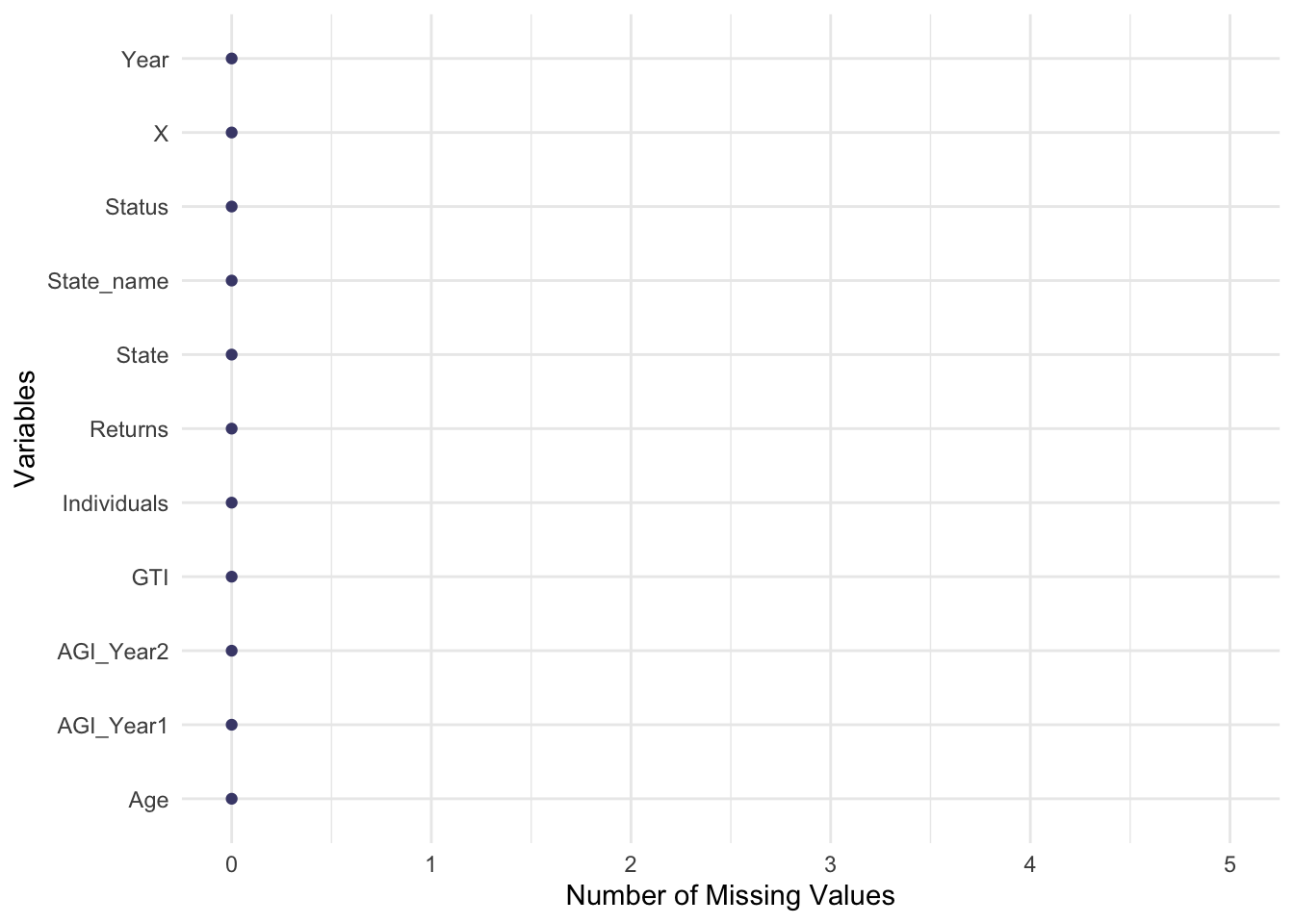
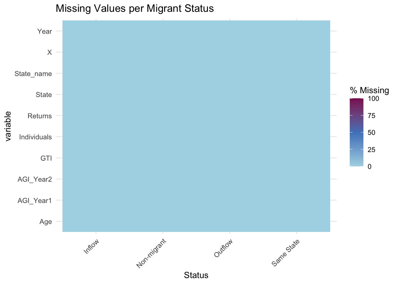
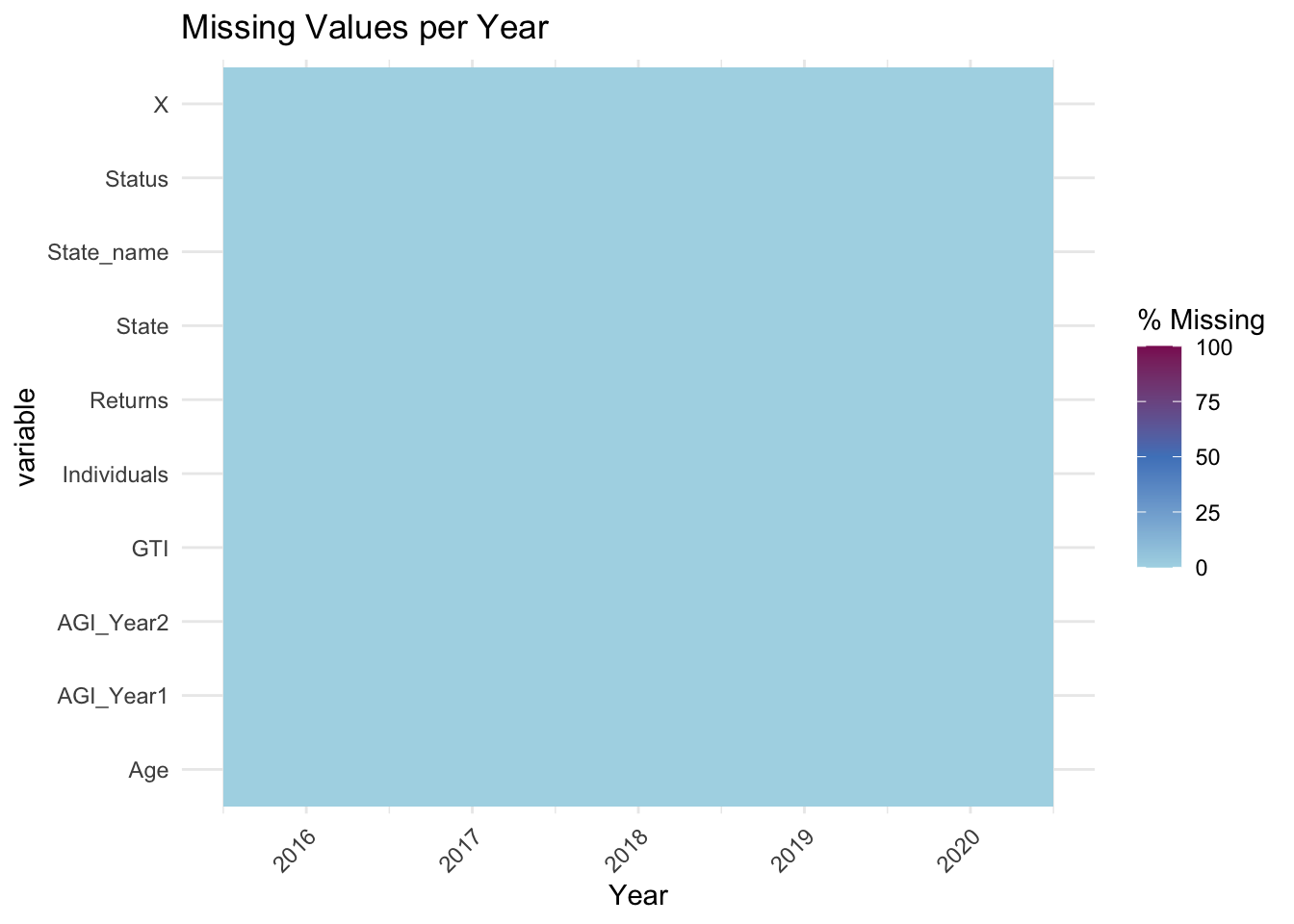
3.3 Missing value analysis
The data available on the IRS website for our analysis does not include any missing values. Data has been aggregated at a total number of returns levels and organized in a way that no values are missing.
Initially, we saw an indication of values being imputted with zero, but as the analysis progressed we noticed that these had a legally sound reason for the true value to be zero.
Below, you can see the landscape of our data for missing values.